Tutorial: Finding and Assigning Peaks in Task-Related fMRI Analysis using Qunex
Brain activity data inferred from functional MR images (fMRI) are stored in a huge voxel space when acquired, resulting in heavy computational operations and cumbersome data analysis, if no other data reduction approaches are applied. The first common approach to data reduction is to project cortical brain activity onto a two-dimensional surface, since neuronal activity should only "light up" within the layers of thin cortical gray matter, and with the spatial resolution limits of modern MRI scanners, a single voxel usually spans all of these layers, so a single voxel is sufficient to model cortical activity. Including a large set of voxels to represent the "inactivity" of the white matter is also an unnecessary waste of space.
Furthermore, not all brain regions are active at the times of interest, and some regions are not of any interest to us, so additional data reduction could be achieved by empirically identifying important brain regions. In Qu|Nex, this is computed with watershed segmentation of brain activity by first identifying the peaks of brain activity and then determining the boundaries of the corresponding activated regions of interest (ROIs). By analyzing ROIs, the span of statistical analyses is reduced from the entire voxel space to specific regions of activation.
In this tutorial, we will demonstrate how this is accomplished in the Qu|Nex environment using the general_find_peaks function, which performs empirical ROI identification on both surface structures, i.e., the cortical sheet, and on the subcortical gray matter modeled with voxels. A detailed reference of the general_find_peaks function and its arguments can be found on the Qu|Nex wiki and we suggest using it alongside this tutorial.
Data Information
To demonstrate the utility of the general_find_peaks, we used data collected in a spatial working memory study, previously presented in Purg et al. (2022). The analysis included 37 healthy young adults (20 women, 19-30 years old), who performed a spatial working memory task while we measured their brain activity with fMRI. The task consisted of a brief presentation of a target stimulus (red disk, 0.1 s), followed by a masking pattern (0.05 s). Participants were asked to remember the position of the target stimulus and, after 10 s of delay, to give a response by moving a probe (gray disk) to the position of the previously presented target by using a joystick. The task design is shown in Figure 1A. MRI data were collected with Philips Achieva 3.0T TX scanner. T1- and T2-weighted structural images were acquired for each participant, while brain activity was measured using BOLD images with T2*-weighted echo-planar imaging sequence.
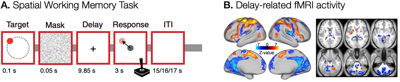
For the purposes of this tutorial, we will use the image of the group-level significant delay-related fMRI cortical and subcortical activity map shown in Figure 1B. You can download the file to follow along.
Peak Identification
Here, we will show a few examples of an empirical ROI analysis on the input image described previously. We will not describe every parameter in detail, because we believe that the details are nicely covered on the function's documentation page. Instead, we will focus on the parameters that are commonly manipulated to achieve desired results.
First, we will look at two basic examples of how to perform ROI analysis on thresholded (Figure 2A) and un-thresholded (Figure 2B) brain maps.
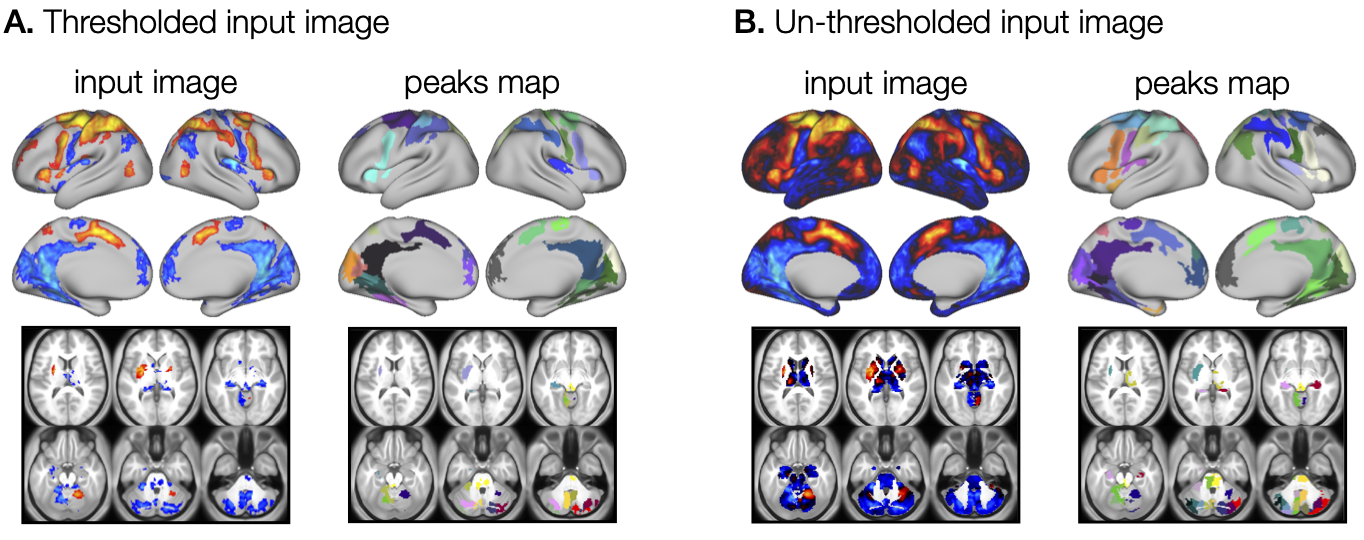
t argument can be set to 0, which indicates that no additional thresholding should be done on the data. B. For un-thresholded brain maps, the t argument can be set to the desired threshold level, where the value reflects the variables stored in the brain map (e.g. Z-scores, p-values). Different colors in the peaks maps represent different ROIs identified with general_find_peaks.The general_find_peaks function supports both types of inputs and it includes an option to threshold the input image before computing ROIs. The thresholding is specified by two parameters, the thresholding level t and val parameter, which defined the direction. Specifically, val='p' removes values smaller than a positive threshold, val='n' removes values greater than a negative threshold, and val='b' removes values lower than the absolute value of t, thresholding data in both directions. The latter is the case in the examples presented here. The peaks map of the thresholded image was computed by running:
qunex general_find_peaks \
	--fin="input_z_scores.dscalar.nii" \
	--fout="output_peaks_map.dscalar.nii" \
	--mins=[300,250] \
	--val="b" \
	--t=0 \
	--presmooth=fwhm:2 \
	--options="limitvol:1"
The peaks map of the un-thresholded image was computed by running a similar command as shown above, except that the thresholding level was set to the desired value of 2.39, as shown below:
qunex general_find_peaks \
	--fin="input_z_scores.dscalar.nii" \
	--fout="output_peaks_map.dscalar.nii" \
	--mins=[300,250] \
	--val="b" \
	--t=2.39 \
	--presmooth=fwhm:2 \
	--options="limitvol:1"
In the second step of the tutorial, we focus on the mins and maxs parameters, which define the minimum and maximum ROI size, respectively. Both parameters are usually defined as two-element vectors, where the first element describes the size in voxels of the regions in the subcortical (volume) structures, and the second element defines the area (mm^2) of the regions on the cortical (surface) structures. Both parameters can be passed to the function as a scalar value, in which case, the same value would be used for surface and volume data. The results of three different size definitions are shown in Figure 3.
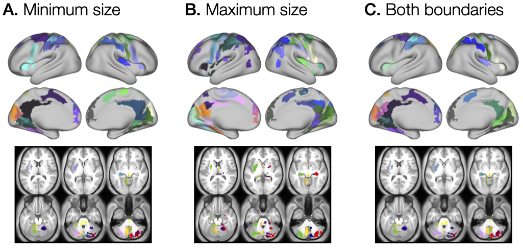
The image shown in Figure 3A was computed by running the command, where only the minimum ROI size was defined, but not restricting their maximum size:
qunex general_find_peaks \
	--fin="input_z_scores.dscalar.nii" \
	--fout="output_peaks_map.dscalar.nii" \
	--mins=[300,250] \
	--val="b" \
	--t=0 \
	--presmooth=fwhm:2 \
	--options="limitvol:1"
The effect of specifying the minimum size is clearly seen as the presence of many small regions in Figure 3B when compared to Figure 3A, where only the maximum ROI size restriction was defined. The image shown in Figure 3B was computed by running:
qunex general_find_peaks \
	--fin="input_z_scores.dscalar.nii" \
	--fout="output_peaks_map.dscalar.nii" \
	--maxs=[300,250] \
	--val="b" \
	--t=0 \
	--presmooth=fwhm:2 \
	--options="limitvol:1"
The image shown in Figure 3C was obtained by restricting both minimum and maximum size ROIs and was computed by running:
qunex general_find_peaks \
	--fin="input_z_scores.dscalar.nii" \
	--fout="output_peaks_map.dscalar.nii" \
	--mins=[300,250] \
	--maxs=[600,500] \
	--val="b" \
	--t=0 \
	--presmooth=fwhm:2 \
	--options="limitvol:1"
Using minimum and maximum size restrictions resulted in the lowest number of identified ROIs.
In the third example, we will demonstrate the usefulness of a parameter for selecting how ROIs are depicted on the brain map. This is controlled by the boundary type in the options parameter. Specifically, we can choose whether the peak map presents only the ROIs (Figure 4A), which are usually neighboring and can be sometimes hard to tell apart visually, or we can define whether to exclude (Figure 4B) or highlight (Figure 4C) the boundary, as well as depict only the boundaries (Figure 4D).
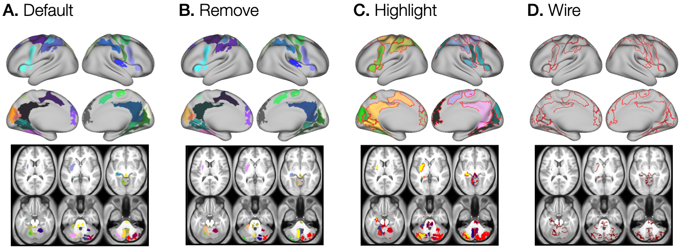
general_find_peaks function provides four different types of ROI visualization, A. the default, B. the remove that excludes grayordinates/voxels at the ROI boundaries, C. the highlight that shows ROI areas and boundaries, and D. the wire to show just ROI boundaries.The peak map shown in Figure 4A is the same peak map shown in Figure 3A, where no boundary parameter was set, hence by default, the map shows no specific boundaries.
The peak map with excluded boundary grayordinates/voxels is shown in Figure 4B and was computed by setting the options parameter to boundary:remove, as shown below.
qunex general_find_peaks \
	--fin="input_z_scores.dscalar.nii" \
	--fout="output_peaks_map.dscalar.nii" \
	--mins=[300,250] \
	--val="b" \
	--t=0 \
	--presmooth=fwhm:2 \
	--options="boundary:remove|limitvol:1"
The peak map with highlighted boundary grayordinates/voxels, which were set to a negative value in order to tell them apart more easily from other ROI data points, is shown in Figure 4C and was computed by setting the options parameter to boundary:highlight, as shown below:
qunex general_find_peaks \
	--fin="input_z_scores.dscalar.nii" \
	--fout="output_peaks_map.dscalar.nii" \
	--mins=[300,250] \
	--val="b" \
	--t=0 \
	--presmooth=fwhm:2 \
	--options="boundary:highlight|limitvol:1"
The peak map that only includes the boundaries of the computed ROIs can be obtained by defining the options parameter to boundary:wire and is shown in Figure 4C. The map was obtained by running:
qunex general_find_peaks \
	--fin="input_z_scores.dscalar.nii" \
	--fout="output_peaks_map.dscalar.nii" \
	--mins=[300,250] \
	--val="b" \
	--t=0 \
	--presmooth=fwhm:2 \
	--options="boundary:wire|limitvol:1"
Each call to the general_find_peaks function produces the output peak map and a tab-separated peak information output in a .txt file. Below is a shortened output from the example shown in Figure 3A:
#source: input_z_scores.dscalar.nii
#mins: [300 250], maxs: Inf, val: 'b', t: 0.0
presmooth.fwhm: 2.0

Component	Label	Peak_value	Avg_value	Size	Area_mm2	Grayord	Peak_x	Peak_y	Peak_z	Centroid_x	Centroid_y	Centroid_z	Wcentroid_x	Wcentroid_y	Wcentroid_z
cerebellum_right	5	-5.9	-2.8	606	NA	75763	  4.0	-54.0	-50.0	  7.8	-53.9	-47.0	  3.7	-52.1	-45.3
brain_stem		6	-6.2	-3.6	527	NA	63458	  0.0	-32.0	-12.0	  1.6	-30.3	-25.7	  1.6	-30.4	-25.1
cerebellum_left		10	-5.8	-4.3	326	NA	73261	-16.0	-62.0	-18.0	-14.4	-60.4	-16.6	-14.5	-60.2	-16.5
cerebellum_left		11	-5.5	-4.0	387	NA	66668	-20.0	-46.0	-52.0	-19.7	-45.7	-52.0	-19.6	-45.6	-52.0
putamen_left		14	7.0	4.8	543	NA	87477	-26.0	  0.0	  4.0	-28.3	 -2.6	  2.1	-28.2	 -2.6	  2.2
hippocampus_left	15	-5.2	-4.0	344	NA	84977	-22.0	-24.0	-14.0	-26.2	-25.2	-12.1	-26.2	-25.3	-12.0
cortex_left		16	-7.2	-5.058	291	251.167	279	-16.842	-52.779	4.728	NA	NA	NA	NA	NA	NA
cortex_left		17	-6.4	-4.670	565	460.073	24729	-22.901	-41.092	-10.801	NA	NA	NA	NA	NA	NA
...
cortex_left		29	-5.4	-3.817	294	269.887	26226	-5.178	52.269	28.303	NA	NA	NA	NA	NA	NA
cortex_right		30	-7.1	-4.990	1257	911.801	29900	8.896	-52.331	7.799	NA	NA	NA	NA	NA	NA
cortex_right		31	-6.3	-4.743	336	257.359	30017	21.330	-48.383	2.580	NA	NA	NA	NA	NA	NA
cortex_right		32	-6.2	-4.256	891	669.650	33316	18.551	-31.452	61.728	NA	NA	NA	NA	NA	NA
The output table contains the properties for every identified region in the peaks map image, such as the maximum activity value of the region (the peak), the average activity, the size of the region, as well as the centroids and weighted centroids of the regions in the volumes structures. The centroids of the regions in the surface structures are not computed, as the surfaces are modeled with a triangular mesh in a 3-dimensional space, and defining a meaningful centroid in the XYZ coordinate space is not straightforward.
Extraction of p-values
The significance of the identified regions of interest can be investigated by extracting the values at the locations of the peaks of regions from a corresponding significance image (e.g. input_p_values.dscalar.nii). The resulting textual output from general_find_peaks is passed as an input and expanded by the general_get_peak_values function as shown below.
general_get_peak_values("output_peaks_map.txt",'input_p_values.dscalar.nii',"output_pval_map.dscalar.txt");The output text file contains the same columns as the output returned by general_find_peaks, with an appended column containing the values at peak locations in the input image file (e.g. the significance image). In this example, we used an input image containing p-values describing the significance of the brain activity, but general_get_peak_values can be used for extracting any other type of data at peak locations specified in the peak report text file.
Assessment of Atlas Region Overlap
general_find_peaks function allows users to assess the overlap between the empirically identified regions and the desired atlas. Let's look at an example of computing an overlap between the identified ROIs and the HCP-MMP1.0 parcellation (Glasser et al., 2016). This is achieved by including parcels:HCP.Parcelation.LR.dscalar.nii in the options argument of the general_find_peaks function. If the specified atlas is not in the search path, you need to define the complete path to the atlas file. Currently, the function only supports atlases in a .dscalar.nii format (future releases will include .dlabel.nii file format). The example call to asses the overlap is shown below:
# ... cortical
qunex general_find_peaks \
	--fin="input_z_scores.dscalar.nii" \
	--fout="output_peaks_map.dscalar.nii" \
	--mins=[300,250] \
	--val="b" \
	--t=0 \
	--presmooth=fwhm:2 \
	--options="parcels:HCP.Parcelation.LR.dscalar.nii|limitvol:1"
And the output text file shows the overlap between ROIs and the HCP atlas:
#source: sWM_delay_Zscores_clustere_fwe_p0.017_peaks.dscalar.nii

frame	ROI	volume_structure	num_vox	perc_vox
1	1	cerebellum_right	533	100.0
1	2	cerebellum_right	630	100.0
1	3	cerebellum_right	411	100.0
...
1	13	cerebellum_left	608	100.0
1	14	putamen_left	543	100.0
1	15	hippocampus_left	344	100.0


frame	ROI	atl_val	num_vox	perc_vox
1	1	0	533	100.0
1	2	0	630	100.0
1	3	0	411	100.0
...
1	18	1015	64	6.6
1	18	1030	75	7.7
1	18	1031	164	16.9
...
1	42	2088	8	1.1
1	42	2097	1	0.1
1	42	2098	8	1.1
The first table in the output file shown above lists the overlap between the identified ROIs in the volume structures and the subcortical segmentation of the CIFTI files. In this example, the overlap was 100% for every subcortical region, because we included limitvol:1 options parameter, which limits the growth of peak regions to the subcortical structure where the peak of the region was found. For example, if the peak (the highest activity) of a region is located on the medial side left thalamus, the growth of the region from its peak is restricted from growing into the right thalamus or any other neighboring subcortical regions.
The second table lists the overlap between the ROIs and the parcels defined in the input atlas image, in our case the HCP parcellation. If we were only interested in the overlap with the CIFTI subcortical structures, we would change the options parameter to parcels:volume.
# ... subcortical
qunex general_find_peaks \
	--fin="input_z_scores.dscalar.nii" \
	--fout="output_peaks_map.dscalar.nii" \
	--mins=[300,250] \
	--val="b" \
	--t=0 \
	--presmooth=fwhm:2 \
	--options="parcels:volume|limitvol:1"
Summary
In this brief tutorial, we covered an example use of the general_find_peaks Qu|Nex function for empirically identifying regions of interest of the fMRI brain activity. We focused on the most commonly varied parameters and did not dive into details and every capability of the function because we believe that the official Qu|Nex documentation covers this well. Additional functionalities, such as details about data smoothing, etc., are also nicely covered in the documentation.
We hope that by using the tutorial alongside the documentation, users are able to obtain a better understanding of the functionalities and the purposes of performing ROI analyses in their research.
References
Glasser, M. F., Coalson, T. S., Robinson, E. C., Hacker, C. D., Harwell, J., Yacoub, E., et al. (2016). A multi-modal parcellation of human cerebral cortex. Nature 536, 171–178. doi:10.1038/nature18933
Purg, N., Starc, M., Slana Ozimič, A., Kraljič, A., Matkovič, A., and Repovš, G. (2022). Neural Evidence for Different Types of Position Coding Strategies in Spatial Working Memory. Frontiers in Human Neuroscience, 16:821545. doi: 10.3389/fnhum.2022.821545