Empirically determining slice acquisition order of Philips Achieva MultiBand BOLD sequences
Introduction
Slice timing correction is an important step in the preprocessing of fMRI data, especially for longer (> 1 s) repetition times (TRs) where the time difference between consecutive slices is larger. Slice timing correction is a temporal data interpolation across all slices in a volume to a common time point. Without slice timing correction, the data is analyzed under the assumption that all voxels were acquired simultaneously. This may be a reasonable assumption for images with very short TRs (< 1 s), which can be obtained with accelerated sequences such as those utilizing multi-slice acquisition (MultiBand) and in-plane acceleration (SENSE). Thus, slice timing correction is usually omitted in such cases. In contrast, images with longer TRs consist of slices for which acquisition is more spread out in time, which can significantly affect the validity of the analysis if not adjusted for. Regardless of TR, many authors suggest that slice timing correction should be performed whenever possible because it leads to better signal quality, even when very fast sequences are used [1,2].
Before proceeding, I strongly recommend reading a previous blog post that describes in more detail what slice timing correction is, why it should be performed, and how to perform it in QuNex.
Determining the slice acquisition order
Slice acquisition strategies for non-accelerated sequences usually follow an interleaved acquisition order from the bottom of the image to the top, e.g., slices 1, 3, 5, 7,... are acquired first, followed by slices 2, 4, 6, 8,... Since different strategies can be used due to various sequence settings and scanner models, it is advisable to get the exact slice timing information instead of just assuming which strategy was used in BOLD sequence in your study. If the DICOM header in your data contains the relevant information on slice order, as is the case with Siemens scanners [3], you can proceed with the correction. Otherwise, you will have to find another way to determine the actual order of the slice acquisition.
At the Mind and Brain Lab in Ljubljana, we use the Philips Achieva 3.0T TX (2011 model) with a dStream upgrade (2020, software release 5.7.1.2.) located at the Faculty of Medicine, Institute of Clinical Physiology. To perform BOLD imaging comparable to contemporary trends in fMRI research, especially images with short TRs to obtain richer temporal information, we utilize both SENSE and MultiBand acquisition acceleration.
Philips scanners provide some slice timing information in the help menu of the control console, describing how various non-accelerated sequences are acquired, along with a few other exceptions, none of which describe the MultiBand case. As mentioned earlier, the simplest solution in such situations would be to avoid slice timing correction and accept the resulting loss of quality. However, this is not acceptable in some situations. An example is the acquisition of fMRI data with very high spatial resolution, where TRs are longer regardless of different acceleration methods due to the large number of slices forming a volume.
Since we could not find information about slice timing for our Philips data anywhere, we decided to find it the "hard way" by empirically determining the slice acquisition order with a seemingly silly experiment in which I continuously rotated my head left and right during fMRI acquisition. In this way, we were able to infer the correct slice acquisition order from the measured angle between the rostral-caudal axis of the head and the vertical axis of each slice (Figure 1A). Since my head was at a different angle at each time point during the acquisition of a volume, slices acquired at different times should be rotated by a different angle, whereas slices acquired at the same time should be at exactly the same angle.
In our experiment, we acquired axial slices from top to bottom. As can be seen in Figures 1 B and 1 C, the most inferior slice is at the top left and the most superior in the bottom right corner.
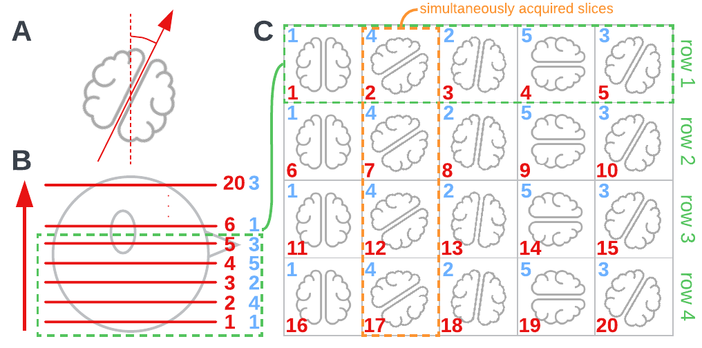
The red numbers in Figure 1 C indicate the position of the slice from bottom to top, whereas the blue numbers indicate the order in which the slice was acquired (e.g., 1 indicates that the slice was acquired first, 2 second, etc.). The same numbering applies to all figures in this post. The number of rows in the figures is adjusted so that slices acquired at the same time are always in the same column, as highlighted by the orange box in Figure 1 C, and the two green boxes indicate a block of slices where each slice was acquired at a different time. The number of such rows in a volume corresponds to the MultiBand factor or the number of simultaneously acquired slices per acquisition. In other words, each column contains the slices that were acquired at the same time. Such an organization allows us to better observe the acquisition strategy.
Results and Discussion
We have performed the experiment with the following five sequence settings to see how different parameters affected the slice acquisition strategy:
- MultiBand 4, SENSE 2, 2.4 mm isometric voxels, 60 axial slices, TR=1000 ms
15 sets of 4 simultaneously acquired slices - MultiBand 4, SENSE 2, 1.8 mm isometric voxels, 76 axial slices, TR=2500 ms
19 sets of 4 simultaneously acquired slices - MultiBand 3, SENSE 2, 2.4 mm isometric voxels, 60 axial slices, TR=1300 ms
20 sets of 3 simultaneously acquired slices - MultiBand 4, SENSE 2, 1.8 mm isometric voxels, 80 axial slices, TR=2500 ms
20 sets of 4 simultaneously acquired slices - MultiBand 4, SENSE 2, 2.0 mm isometric voxels, 72 axial slices, TR=2000 ms, 18 sets of 4 simultaneously acquired slices
The results are presented in a matrix of axial slices in the format described in Figure 1 C.
In the first sequence, shown in Figure 2, each volume consisted of 60 axial slices, and we used a MultiBand factor of 4, meaning that a volume consisted of 4 rows of 15 slices; therefore 15 sets of 4 simultaneously acquired slices.
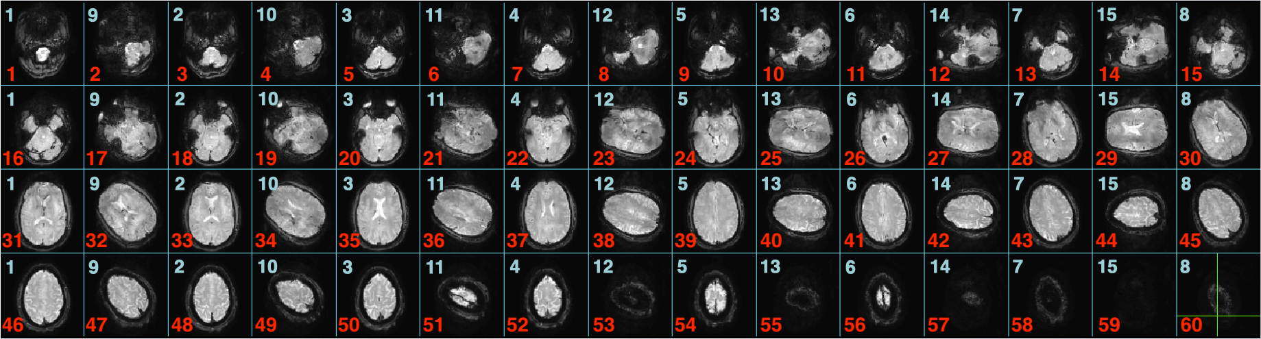
In the first sequence, we noticed that each of the four rows of 15 slices followed an interleaved slice acquisition strategy. More specifically, the odd slices (red numbers) were acquired first (1, 3, 5, 7, 9, 11, 13, 15), followed by the even slices (2, 4, 6, 8, 10, 12, 14).
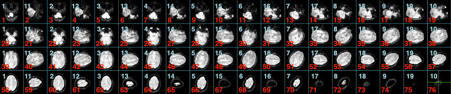
A similar pattern was observed in the second sequence shown in Figure 3, which consisted of 76 axial slices acquired with a MultiBand factor 4, resulting in 19 sets of 4 simultaneously acquired slices. Similarly to the first sequence, in the second sequence, the odd slices (1, 3, 5, 7, 9, 11, 13, 15, 17, 19) were acquired first, followed by the even slices (2, 4, 6, 8, 10, 12, 14, 16, 18).
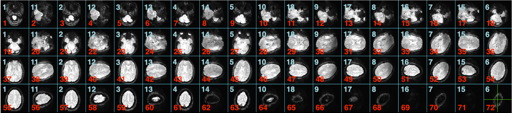
A surprising pattern was observed in the third and fourth sequences, where a different, more complex acquisition pattern was observed. The results of the third pattern are shown in Figure 4, which was acquired with a MultiBand factor 3. Thus, the image consisted of 20 sets of 3 simultaneously acquired slices.
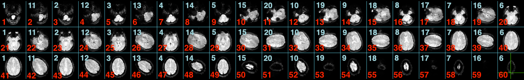
In the third case, the slices were acquired in the following order: 1, 3, 5, 7, 9, 20, 18, 16, 14, 12, 2, 4, 6, 8, 10, 19, 17, 15, 13, 11.
This acquisition strategy is clearly more complicated than the strategy in the first two cases. The only common factor that seemed to be the reason for a different acquisition strategy in the third sequence was the number of slices within each row, specifically whether that number was even or odd. In the first two cases, rows consisted of 19 and 15 slices (odd), whereas in the third case, the rows consisted of 20 slices (even). To verify whether this assumption was true, we acquired the fourth sequence with 80 axial slices and MultiBand factor 4, resulting in 20 slices per row (even). The acquisition strategy in the fourth example, shown in Figure 5, was similar to the third case and followed the same complicated order (1, 3, 5, 7, 9, 20, 18, 16, 14, 12, 2, 4, 6, 8, 10, 19, 17, 15, 13, 11).

In the third and fourth sequences, the odd slices in the first half of the row are acquired first up until the half of the row, followed by the even slices in the second half, acquired in reverse order (from the uppermost slice in the row to the slice in the middle of the row, then come the even slices in the first half, acquired upward, and finally the odd slices in the second half acquired downward towards the middle.
With the fifth sequence, we wanted to analyze whether the strategy changes when the number of slices in a row is even but not divisible by four, i.e., when half of the row does not contain an even number of slices. For example, the third and fourth sequences consisted of rows with 20 slices, resulting in two halves of 10 slices, an even number. We suspected that in cases where the number of slices in a row was not divisible by 4, a different strategy might be adopted, as in the fifth case with 18 slices per row, where each half consisted of 9 slices. The results of the fifth sequence are shown in Figure 6.
The strategy seemed to be very similar to the previous cases when the number of slices in a row was even, except that we had to derive a slightly different empirical equation for calculating the slice timing order. If you look closely, the acquisition order of the slices in the middle of the row is slightly different when the number of slices in one half of the row is odd. For example, in the third and fourth cases, the middle-most slice in the second half of the row is acquired last, while in the fifth case, the first slice above the middle-most one is acquired last.
Python script for creating slice timing correction input files
We created the attached Python script to compute the slice timing order and generate slice timing files used by QuNex during fMRI preprocessing.
For example, to create a slice order file slice_timing_MB4.txt for a sequence with 60 slices and MultiBand factor 4 (first sequence described earlier) run:
python prepare_philips_multiband_slice_order_file.py \
    --number_of_slices 60 \
    --multiband_factor 4 \
    --output_file_name slice_timing.txt
From then on, we can use the generated slice timing correction file in QuNex preprocessing by following the steps described in the previously mentioned QuNex tutorial.
The method used in the script is not a mechanistically correct solution for calculating the slice timing strategy, but it is an empirically derived method that works for the sequence examples presented in this post.
Summary
This blog post explores the importance of slice timing correction in preprocessing fMRI data, particularly for longer repetition times (TRs). It introduces an empirical method for determining the slice acquisition order by measuring angular variations during subject head rotation. The post discusses experimental results involving different acquisition settings that reveal both interleaved and more complex acquisition patterns. We emphasize the importance of accurate slice timing correction and provide a Python script for creating slice timing order files that can be used in QuNex fMRI data preprocessing. This practical approach shows promise for improving the validity and quality of fMRI data.
Please note that these acquisition strategies may not be universally applicable to all Philips scanners, as they may vary depending on specific sequence settings and scanner software versions. While providing valuable insights, we strongly recommend that users validate their data's slice acquisition order. This can be done either by performing an experiment similar to the one described in this post or by comparing the quality of slice timing-corrected data to uncorrected data.
Speaking of which, an analysis of the improvements in image quality by the proposed method should also be performed on our part. This additional step could further validate these findings and assess the extent of the benefits of slice timing correction in sequences with longer TRs. This seems like a promising premise for a potential sequel post.
I welcome contributions and insights from those who have explored slice acquisition order in Philips MultiBand sequences. If anyone identifies potential errors in my analysis or reasoning, I would greatly appreciate your input (my contact information).